QGIS 2.1x is a brilliant tool for Python-based automation in form of custom scripts or even plugins. The first steps towards writing the custom code might be a bit difficult, as you need to grasp quite complex Python API. The QGIS Plugin Development series (see the list of other parts at the end of this article) targets pitfalls and traps I’ve met while learning to use it myself.
The outcome of the series is going to be a fully functional custom plugin capable of writing attribute values from a source layer nearest neighbour to a target layer based on their spatial proximity.
In this part, I’ll mention the basics a.k.a. what is good to know before you start.
Documentation
Different QGIS versions come with different Python API. The documentation is to be found at https://qgis.org, the latest being version 2.18. Note that if you come directly to http://qgis.org/api/, you’ll see the current master docs.
Alternatively, you can apt install qgis-api-doc on your Ubuntu-based system and run python -m SimpleHTTPServer [port] inside /usr/share/qgis/doc/api. You’ll find the documentation at http://localhost:8000 (if you don’t provide port number) and it will be available even when you’re offline.
Basic API objects structure
Before launching QGIS, take a look at what’s available inside API:
- qgis.core package brings all the basic objects like QgsMapLayer, QgsDataSourceURI, QgsFeature etc
- qgis.gui package brings GUI elements that can be used within QGIS like QgsMessageBar or QgsInterface (very important API element, exposed to all custom plugins)
- qgis.analysis, qgis.networkanalysis, qgis.server, and qgis.testing packages that won’t be covered in the series
- qgis.utils module that comes with
iface exposed (very handy within QGIS Python console)
QGIS Python Console
Using Python console is the easiest way to automate your QGIS workflow. It can be accessed via pressing Ctrl + Alt + P or navigating to Plugins -> Python Console. Note the above mentioned iface from qgis.utils module is exposed by default within the console, letting you interact with QGIS GUI. Try out the following examples.
iface.mapCanvas().scale() # returns the current map scale
iface.mapCanvas().zoomScale(100) # zoom to scale of 1:100
iface.activeLayer().name() # get the active layer name
iface.activeLayer().startEditing() # toggle editting
That was a very brief introduction to QGIS API, the next part will walk you through the console more thoroughly.
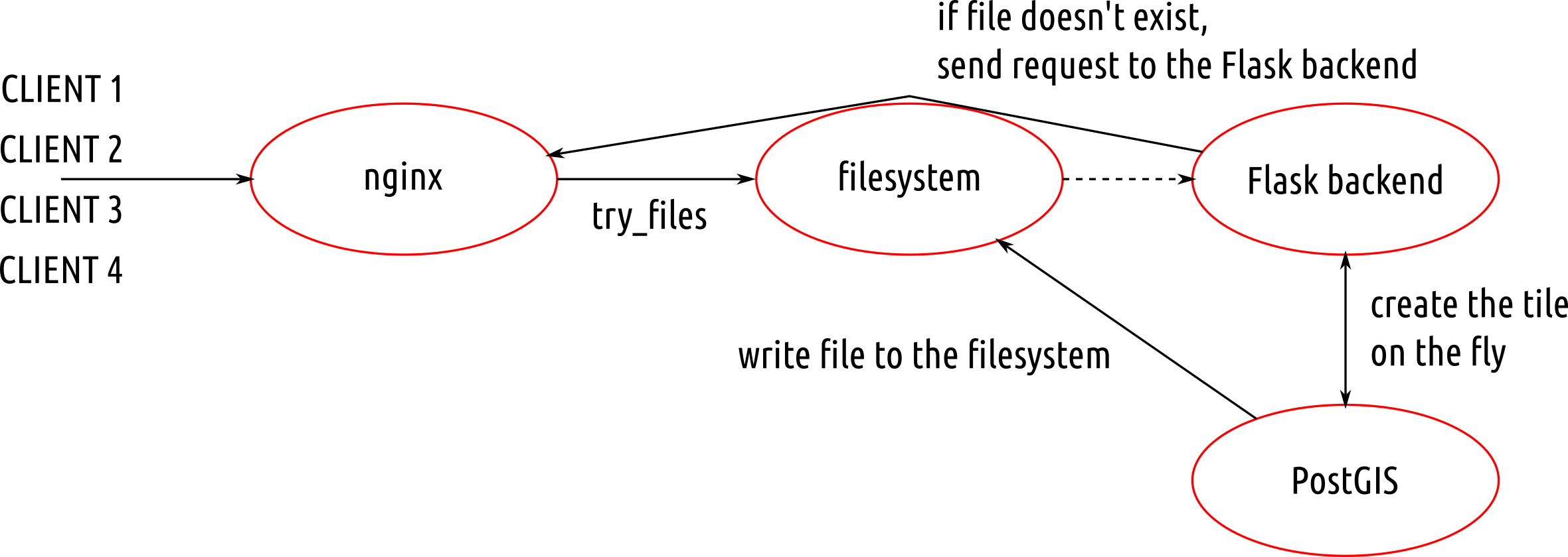
Since version 2.4.0, PostGIS can serve MVT data directly. MVT returning queries put heavy workload on the database though. On top of that, each of the query has to be run again every time a client demands the data. This leaves us with plenty of room to optimize the process.
During the last week, while working on the Czech legislative election data visualization, I’ve struggled with the server becoming unresponsive far too often due to the issues mentioned above.
According to the schema, the first client to come to the server:
- goes through filesystem unstopped, because there are no cached files yet,
- continues to the Flask backend and asks for a file at
{z}/{x}/{y},
- Flask backend asks the database to return the MVT for the given tile,
- Flask backend writes the response to the filesystem and sends it to the client.
Other clients get tiles directly from the filesystem, leaving the database at ease.
Nginx
Nginx is fairly simple to set up, once you know what you’re doing. The /volby-2017/municipality/ location serves static MVT from the given alias directory. If not found, the request is passed to @postgis location, that asks the Flask backend for the response.
server election {
    location /volby-2017/municipality {
            alias /opt/volby-cz-2017/server/cache/;
            try_files $uri @postgis;
    }

    location @postgis {
            include uwsgi_params;
            uwsgi_pass 127.0.0.1:5000;
    }
}
Flask backend
Generating static MVT in advance
If you’re going to serve static tiles that don’t change often, it might be a good idea to use PostGIS to create files in advance and serve them with Nginx.
CREATE TABLE tiles (
    x integer,
    y integer,
    z integer,
    west numeric,
    south numeric,
    east numeric,
    north numeric,
    geom geometry(POLYGON, 3857)
);
Using mercantile, you can create the tiles table holding the bounding boxes of the tiles you need. PostGIS them inserts the actual MVT into the mvt table.
CREATE TEMPORARY TABLE tmp_tiles AS
    SELECT
        muni.muni_id,
        prc.data,
        ST_AsMVTGeom(
            muni.geom,
            TileBBox(z, x , y, 3857),
            4096,
            0,
            false
        ) geom,
        x,
        y,
        z
    FROM muni
    JOIN (
        SELECT
            x,
            y,
            z,
            geom
        FROM tiles
    ) bbox ON (ST_Intersects(muni.geom, bbox.geom))
    JOIN party_results_cur prc ON (muni.muni_id = prc.muni_id);
CREATE TABLE mvt (mvt bytea, x integer, y integer, z integer);
DO
$$
DECLARE r record;
BEGIN
FOR r in SELECT DISTINCT x, y, z FROM tmp_tiles LOOP
    INSERT INTO mvt
    SELECT ST_AsMVT(q, 'municipality', 4096, 'geom'), r.x, r.y, r.z
    FROM (
        SELECT
            muni_id,
            data,
            geom
        FROM tmp_tiles
        WHERE (x, y, z) = (r)
    ) q;
    RAISE INFO '%', r;
END LOOP;
END;
$$;
Once filled, the table rows can be written to the filesystem with the simple piece of Python code.
#!/usr/bin/env python

import logging
import os
import time
from sqlalchemy import create_engine, text

CACHE_PATH="cache/"

e = create_engine('postgresql:///')
conn = e.connect()
sql=text("SELECT mvt, x, y, z FROM mvt")
query = conn.execute(sql)
data = query.cursor.fetchall()

for d in data:
    cachefile = "{}/{}/{}/{}".format(CACHE_PATH, d[3], d[1], d[2])
    print(cachefile)

    if not os.path.exists("{}/{}/{}".format(CACHE_PATH, d[3], d[1])):
        os.makedirs("{}/{}/{}".format(CACHE_PATH, d[3], d[1]))

    with open(cachefile, "wb") as f:
        f.write(bytes(d[0]))
Conclusion
PostGIS is a brilliant tool for generating Mapbox vector tiles. Combined with Python powered static file generator and Nginx, it seems to become the only tool needed to get you going.
I spend a lot of time reading PostgreSQL docs. It occurred to me just a few weeks ago that those versioned manuals are great opportunity to get an insight into PostgreSQL development history. Using PostgreSQL, of course.
TOP 5 functions with the most verbose docs in each version
SELECT
    version,
    string_agg(func, ' | ' ORDER BY letter_count DESC)
FROM (
    SELECT
        version,
        func,
        letter_count,
        row_number() OVER (PARTITION BY version ORDER BY letter_count DESC)
    FROM postgresql_development.data
) a
WHERE row_number <= 10
GROUP BY version
ORDER BY version DESC
Seems like a huge comeback for CREATE TABLE.
| VERSION |
1st |
2nd |
3rd |
4th |
5th |
| 10.0 |
CREATE TABLE |
ALTER TABLE |
REVOKE |
GRANT |
SELECT |
| 9.6 |
REVOKE |
ALTER TABLE |
GRANT |
CREATE TABLE |
SELECT |
| 9.5 |
REVOKE |
ALTER TABLE |
GRANT |
CREATE TABLE |
SELECT |
| 9.4 |
REVOKE |
GRANT |
ALTER TABLE |
CREATE TABLE |
SELECT |
| 9.3 |
REVOKE |
GRANT |
CREATE TABLE |
ALTER TABLE |
ALTER DEFAULT PRIVILEGES |
| 9.2 |
REVOKE |
GRANT |
CREATE TABLE |
ALTER TABLE |
ALTER DEFAULT PRIVILEGES |
| 9.1 |
REVOKE |
GRANT |
CREATE TABLE |
ALTER TABLE |
ALTER DEFAULT PRIVILEGES |
| 9.0 |
REVOKE |
GRANT |
CREATE TABLE |
ALTER TABLE |
ALTER DEFAULT PRIVILEGES |
| 8.4 |
REVOKE |
GRANT |
CREATE TABLE |
ALTER TABLE |
SELECT |
| 8.3 |
REVOKE |
CREATE TABLE |
GRANT |
ALTER TABLE |
COMMENT |
| 8.2 |
REVOKE |
CREATE TABLE |
GRANT |
ALTER TABLE |
SELECT |
| 8.1 |
REVOKE |
CREATE TABLE |
GRANT |
ALTER TABLE |
SELECT |
| 8 |
CREATE TABLE |
REVOKE |
GRANT |
SELECT |
ALTER TABLE |
| 7.4 |
CREATE TABLE |
REVOKE |
ALTER TABLE |
GRANT |
SELECT |
| 7.3 |
CREATE TABLE |
SELECT |
ALTER TABLE |
REVOKE |
GRANT |
| 7.2 |
CREATE TABLE |
SELECT INTO |
SELECT |
ALTER TABLE |
CREATE TYPE |
| 7.1 |
CREATE TABLE |
SELECT INTO |
SELECT |
CREATE TYPE |
ALTER TABLE |
| 7.0 |
SELECT |
SELECT INTO |
CREATE TYPE |
CREATE TABLE |
COMMENT |
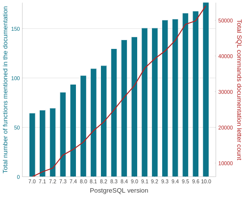
Number of functions available in each version
SELECT
    version,
    count(func),
    sum(letter_count)
FROM postgresql_development.data
GROUP BY version ORDER BY version;
The most verbose docs in each version
SELECT DISTINCT ON (version)
    version,
    func,
    letter_count
FROM postgresql_development.data
ORDER BY version, letter_count DESC;
Poor REVOKE, the defeated champion.
| VERSION |
FUNCTION |
LETTER COUNT |
| 10 |
CREATE TABLE |
3142 |
| 9.6 |
REVOKE |
2856 |
| 9.5 |
REVOKE |
2856 |
| 9.4 |
REVOKE |
2856 |
| 9.3 |
REVOKE |
2856 |
| 9.2 |
REVOKE |
2856 |
| 9.1 |
REVOKE |
2508 |
| 9 |
REVOKE |
2502 |
| 8.4 |
REVOKE |
2105 |
| 8.3 |
REVOKE |
1485 |
| 8.2 |
REVOKE |
1527 |
| 8.1 |
REVOKE |
1312 |
| 8 |
CREATE TABLE |
1251 |
| 7.4 |
CREATE TABLE |
1075 |
| 7.3 |
CREATE TABLE |
929 |
| 7.2 |
CREATE TABLE |
929 |
| 7.1 |
CREATE TABLE |
871 |
| 7 |
SELECT |
450 |
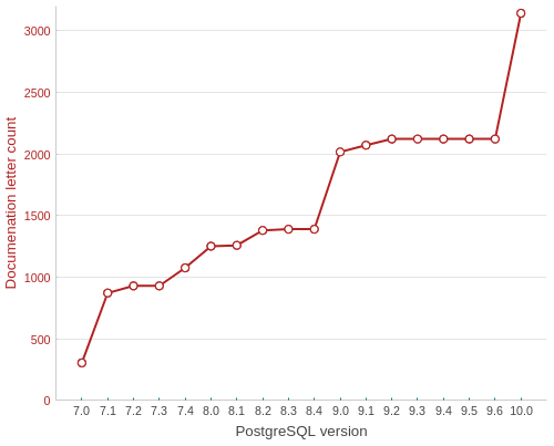
CREATE TABLE docs evolution
SELECT
    version,
    letter_count
FROM postgresql_development.data
WHERE func = 'CREATE TABLE'
ORDER BY func, version;
Something’s going on in an upcoming 10.0 version.
All the data was obtained with the following Python script and processed inside the PostgreSQL database. Plots done with Bokeh, though I probably wouldn’t use it again, the docs site is absurdly sluggish and the info is just all over the place.
As mentioned in QGIS Tips For Collaborative Mapping we’re in the middle of crop evaluation project at CleverMaps.
With the QGIS workflow up and running, I’ve been focused on different QGIS related task: automatic map generation for land blocks that meet certain conditions. The logic behind identifying such land blocks is as follows:
- if the original area and the measured one differ more than 0.5 % or
- number of declared crops differs from number of crops identified or
- at least one parcel in the land block was given a certain error code
Let’s assume that with several lines of SQL code we can store these mentioned above in a table called land_blocks with geometries being the result of calling ST_Union() over parcels for each land block.
Map composition
Every map should feature following layers:
- land blocks (remember the
land_blocks table?) - labeled with ID, yellowish borders, no fill
- land parcels - that’s my source layer - labeled with letters, blue borders, no fill
- other layers
- HR, VHR, NIR imagery, orthophoto - served via WMS
Labels should be visible only for the featured land block (both for the land parcels and the land block itself. The whole map scales dynamically, showing small land blocks zoomed in and the large ones zoomed out.

Every map features additional items:
- dynamic list of subsidies farmer asks for - showing both measured and declared area
- dynamic list of land parcels with their areas and error codes
- scalebar
- map key
- logos
Atlas creation
Now with requirements defined, let’s create some maps. It’s incredibly easy to generate a series of maps with QGIS atlas options.
Atlas generation settings
Coverage layer is presumably the only thing you really need - as the name suggests, it covers your area of interest. One map will be created for each feature in this layer, unless you decide to use some filtering - which I did.
Output filenames can be tweaked to your needs, here’s what such a function might look like. If there is a slash in the land block ID (XXXXXXX/Y), the filename is set to USER-ID_XXXXXXX-00Y_M_00, USER-ID_XXXXXXX-000_M_00 otherwise.
CASE WHEN strpos(attribute($atlasfeature, 'kod_pb'), '/') > -1
    THEN
        ji || '_' ||
        substr(
            attribute($atlasfeature, 'kod_pb'), 0,
            strpos(attribute($atlasfeature, 'kod_pb'), '/')+1 -- slash position
        ) || '-' ||
        lpad(
            substr(
                attribute($atlasfeature, 'kod_pb'),
                strpos(attribute($atlasfeature, 'kod_pb'), '/') + 2,
                length(attribute($atlasfeature, 'kod_pb'))
            ),
        3, '0') || '_M_00'
    ELSE
        ji || '_' || attribute($atlasfeature, 'kod_pb') || '-000_M_00'
END
Map scale & variable substitutions
Different land blocks are of different sizes, thus needing different scales to fit in the map. Again, QGIS handles this might-become-a-nightmare-pretty-easily issue with a single click. You can define the scale as:
- margin around feature: percentage of the space displayed around
- predefined scale (best fit): my choice, sometimes it doesn’t display the entire land block though
- fixed scale: sets the scale the same for all the maps
With these settings, I get a map similar to the one below. Notice two interesting things:

- Scale uses decimal places, which I find a huge failure. Has anyone ever seen a map with such scale? The worst is there is no easy way to hide these, or at least I didn’t find one.
- You can see a bunch of
[something in the brackets] notations. These will be substituted with actual values during the atlas generation. Showing land block ID with a preceeding label is as easy as [%concat('PB: ', "kod_pb")%] (mind the percentage sign).
Styling the map using atlas features
Atlas features are a great help for map customization. As mentioned earlier, in my case, only one land block label per map should be visible. That can be achieved with a simple label dialog expression:
CASE
    WHEN $id = $atlasfeatureid
    THEN "kod_pb"
END
QGIS keeps reference to each coverage layer feature ID during atlas generation, so you can use it for comparison. The best part is you can use IDs with any layer you need:
CASE
    WHEN attribute($atlasfeature, 'kod_pb') = "kod_pb"
    THEN "kod_zp"
END
With this simple expression, I get labels only for those land parcels that are part of the mapped land block. Even the layer style can be controlled with atlas feature. Land parcels inside the land block have blue borders, the rest is yellowish, remember? It’s a piece of cake with rule-based styling.

Atlas generation
When you’re set, atlas can be created with a single button. I used SVG as an output format to easily manipulate the map content afterwards. The resulting maps look like the one in the first picture without the text in the red rectangle. A Python script appends this to each map afterwards.
Roughly speaking, generating 300 maps takes an hour or so, I guess that depends on the map complexity and hardware though.
Adding textual content
SVG output is just plain old XML that you can edit by hand or by script. A simple Python script, part of map post-processing, loads SVG from the database and adds it to the left pane of each map.
SELECT
      ji,
      kod_pb,
      concat(
            '<g fill="none" stroke="#000000" stroke-opacity="1" stroke-width="1"
                  stroke-linecap="square" stroke-linejoin="bevel" transform="matrix(1.18081,0,0,1.18081,270.0,550.0)"
                  font-family="Droid Sans" font-size="35" font-style="normal">',
            kultura, vymery, vymery_hodnoty,
            vcs_titul, vcs_brk, vcs_brs, vcs_chmel,
            vcs_zvv, vcs_zv, vcs_ovv, vcs_ov, vcs_cur, vcs_bip,
            lfa, lfa_h1, lfa_h2, lfa_h3,
            lfa_h4, lfa_h5, lfa_oa, lfa_ob, lfa_s,
            natura, aeo_eafrd_text, dv_aeo_eafrd_a1,
            dv_aeo_eafrd_a2o, dv_aeo_eafrd_a2v, dv_aeo_eafrd_b1,
            dv_aeo_eafrd_b2, dv_aeo_eafrd_b3, dv_aeo_eafrd_b4,
            dv_aeo_eafrd_b5, dv_aeo_eafrd_b6, dv_aeo_eafrd_b7,
            dv_aeo_eafrd_b8, dv_aeo_eafrd_b9, dv_aeo_eafrd_c1,
            dv_aeo_eafrd_c3, aeko_text, dv_aeko_a, dv_aeko_b, dv_aeko_c,
            dv_aeko_d1, dv_aeko_d2, dv_aeko_d3, dv_aeko_d4, dv_aeko_d5,
            dv_aeko_d6, dv_aeko_d7, dv_aeko_d8, dv_aeko_d9, dv_aeko_d10,
            dv_aeko_e, dv_aeko_f, ez, dzes_text, rep, obi, seop, meop, pbz, dzes7,
            '</g>'
      ) popis
FROM (...);
Each column from the previous query is a result of SELECT similar to the one below.
SELECT concat('<text fill="#000000" fill-opacity="1" stroke="none">BrK: ', dv_brk, ' ha / ', "MV_BRK", ' ha;', kod_dpz, '</text>') vcs_brk
The transform="matrix(1.18081,0,0,1.18081,270.0,550.0) part puts the text on the right spot. Great finding about SVG is that it places each <text> element on the new line, so you don’t need to deal with calculating the position in your script.
Scale adjustment is done with a dirty lambda function.
content = re.sub(r">(\d{1,3}\.\d{3,5})</text>", lambda m :"> " + str(int(round(float(m.group(1))))) + "</text>", old_map.read())
SVG to JPEG conversion
We deliver maps as JPEG files with 150 DPI on A4 paper format. ImageMagick converts the formats with a simple shell command:
convert -density 150 -resize 1753x1240 input.svg output.jpg
Conclusion
I created pretty efficient semi-automated workflow using several open source technologies that saves me a lot of work. Although QGIS has some minor pet peeves (scale with decimal places, not showing the entire feature, not substituting variables at times), it definitely makes boring map creation quite amusing. The more I work with big data / on big tasks, the more I find Linux a must-have.
The whole process was done with QGIS 2.10, PostGIS 2.1, PostgreSQL 9.3, Python 2.7, ImageMagick 6.7.