I got my hands on pgRouting in the last post and I’m about to do the same with GRASS GIS in this one.
GRASS GIS stores the topology for the native vector format by default, which makes it easy to use for the network analysis. All the commands associated with the network analysis can be found in the v.net family. The ones I’m going to discuss in this post are v.net itself, v.net.path, .v.net.alloc and v.net.iso, respectively.
Data
I’m going to use the roads data from the previous post together with some random points used as catchment areas centers.
# create the new GRASS GIS location
grass -text -c ./osm/czech

# import the roads
v.in.ogr input="PG:host=localhost dbname=pgrouting" layer=cze.roads output=roads -eo  --overwrite

# import the random points
v.in.ogr input="PG:host=localhost dbname=pgrouting" layer=temp.points output=points -eo --overwrite
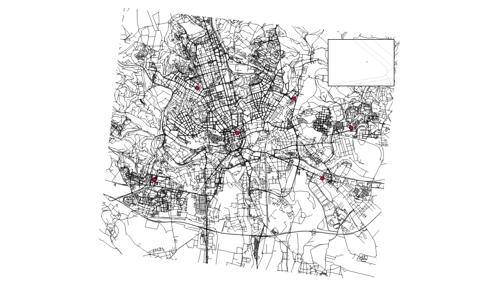
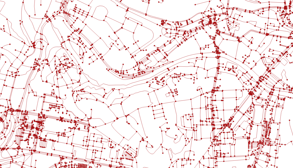
I got six different points and the pretty dense road network. Note none of the points is connected to the existing network.
You have to have routable network to do the actual routing (the worst sentence ever written). To do so, let’s:
- connect the random points to the network
- add nodes to ends and intersections of the roads
Note I’m using the 500m as the max distance in which to connect the points to the network.
v.net input=roads points=points operation=connect threshold=500 output=network
v.net input=network output=network_noded operation=nodes
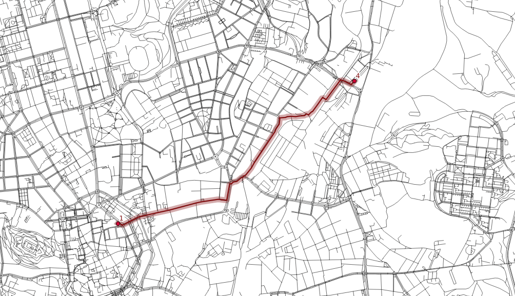
Finding the shortest path between two points
Once the network is routable, it is easy to find the shortest path between points number 1 and 4 and store it in the new map.
echo "1 1 4" | v.net.path input=network_noded output=path_1_4
The algorithm doesn’t take bridges, tunnels and oneways into account, it’s capable of doing so though.
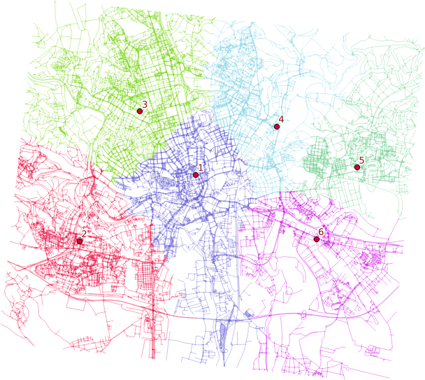
Distributing the subnets for nearest centers
v.net.alloc input=network_noded output=network_alloc center_cats=1-6 node_layer=2
v.net.alloc module takes the given centers and distributes the network so each of its parts belongs to exactly one center - the nearest one (speaking the distance, time units, …).
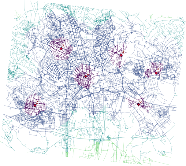
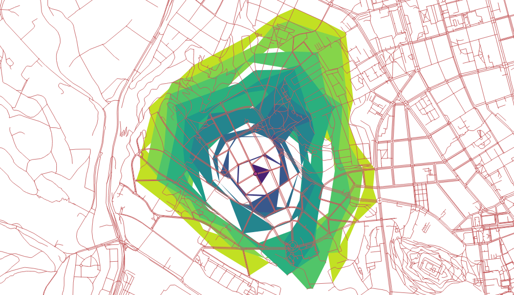
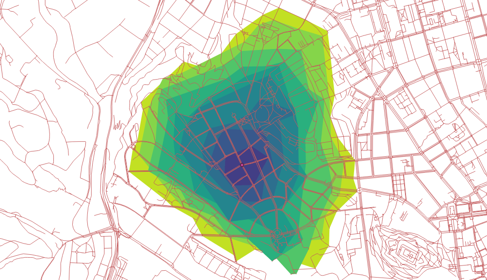
Creating catchment areas
v.net.iso input=network_noded output=network_iso center_cats=1-6 costs=1000,3000,5000
v.net.iso splits net by cost isolines. Again, the costs might be specified as lengths, time units, ….
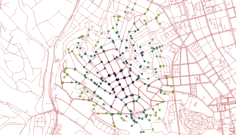
Two different ways lead to the actual catchment area creation. First, you extract nodes from the roads with their values, turn them into the raster grid and either extract contours or polygonize the raster. I find the last step suboptimal and would love to find another way of polygonizing the results.
Note when extracting contours the interval has to be set to the reasonable number depending on the nodes values.
Remarks
- Once you grasp the basics, GRASS GIS is real fun. Grasping the basics is pretty tough though.
- Pedestrians usually don’t follow the road network.
- Bridges and tunnels might be an issue.
- Personally, I find GRASS GIS easier to use for the network analysis compared to pgRouting.
For a long time I’ve wanted to play with pgRouting and that time has finally come. Among many other routing functions there is one that caught my eye, called pgr_drivingdistance. As the documentation says, it returns the driving distance from a start node using Dijkstra algorithm. The aforementioned distance doesn’t need to be defined in Euclidean space (the real distance between two points), it might be calculated in units of time, slopeness etc. How to get it going?
Data
OSM will do as it always does. There is a tool called osm2pgrouting to help you load the data, the pure GDAL seems to be a better way to me though. Importing the downloaded data is trivial.
ogr2ogr -f "PostgreSQL" PG:"dbname=pgrouting active_schema=cze" \
-s_srs EPSG:4326 \
-t_srs EPSG:5514 \
roads.shp \
-nln roads \
-lco GEOMETRY_NAME=the_geom \
-lco FID=id \
-gt 65000� \
-nlt PROMOTE_TO_MULTI \
-clipsrc 16.538 49.147 16.699 49.240
To route the network, it has to be properly noded. Although pgRouting comes with built-in pgr_nodenetwork, it didn’t seem to work very well. To node the network, use PostGIS ST_Node. Note this doesn’t consider bridges and tunnels.
CREATE TABLE cze.roads_noded AS
SELECT
    (ST_Dump(geom)).geom the_geom
FROM (
    SELECT
        ST_Node(geom) geom
    FROM (
        SELECT ST_Union(the_geom) geom
        FROM cze.roads
    ) a
) b;
After noding the network, all the information about speed limits and oneways is lost. If needed, it can be brought back with following:
CREATE INDEX ON cze.roads_noded USING gist(the_geom);
ALTER TABLE cze.roads_noded ADD COLUMN id SERIAL PRIMARY KEY;
ALTER TABLE cze.roads_noded ADD COLUMN maxspeed integer;

UPDATE cze.roads_noded
SET maxspeed = a.maxspeed
FROM (
    SELECT DISTINCT ON (rn.id)
        rn.id,
        r.maxspeed
    FROM cze.roads_noded rn
    JOIN cze.roads r ON (ST_Intersects(rn.the_geom, r.the_geom))
    ORDER BY rn.id, ST_Length(ST_Intersection(rn.the_geom, r.the_geom)) DESC
) a
WHERE cze.roads_noded.id = a.id;
With everything set, the topology can be built.
ALTER TABLE cze.roads_noded ADD COLUMN source integer;
ALTER TABLE cze.roads_noded ADD COLUMN target integer;
SELECT pgr_createTopology('cze.roads_noded', 1);
This function creates the cze.roads_noded_vertices_pgr that contains all the extracted nodes from the network.
As already mentioned, measures other than length can be used as a distance, I chose the time to get to a given node on foot.
ALTER TABLE cze.roads_noded ADD COLUMN cost_minutes integer;
UPDATE cze.roads_noded
SET cost_minutes = (ST_Length(the_geom) / 83.0)::integer; -- it takes average person one minute to walk 83 meters

UPDATE cze.roads_noded
SET cost_minutes = 1
WHERE cost_minutes = 0;
Routing
Now the interesting part. All the routing functions are built on what’s called inner queries that are expected to return a certain data structure with no geometry included. As I want to see the results in QGIS immediately, I had to use a simple anonymous PL/pgSQL block that writes polygonal catchment areas to a table (consider it a proof of concept, not the final solution).
DROP TABLE IF EXISTS cze.temp;
CREATE TABLE cze.temp AS
SELECT *
FROM cze.roads_noded_vertices_pgr ver
JOIN (
    SELECT *
    FROM pgr_drivingDistance(
        'SELECT id, source, target, cost_minutes as cost, cost_minutes as reverse_cost FROM cze.roads_noded',
        6686,
        10,
        true
    )
)dist ON ver.id = dist.node;

DO $$
DECLARE
    c integer;
BEGIN
    DROP TABLE IF EXISTS tmp;
    CREATE TABLE tmp (
        agg_cost integer,
        geom geometry(MULTIPOLYGON, 5514)
    );

    -- order by the biggest area so the polygons are not hidden beneath the bigger ones
    FOR c IN SELECT agg_cost FROM cze.temp GROUP BY agg_cost HAVING COUNT(1) > 3 ORDER BY 1 DESC LOOP
        RAISE INFO '%', c;
        INSERT INTO tmp (agg_cost, geom)
        SELECT
            c,
            ST_Multi(ST_SetSRID(pgr_pointsAsPolygon(
                'SELECT
                        temp.id::integer,
                        ST_X(temp.the_geom)::float AS x,
                        ST_Y(temp.the_geom)::float AS y
                FROM cze.temp
                WHERE agg_cost = ' || c
            ), 5514));
    END LOOP;
END$$;
Using pgr_pointsAsPolygon renders resulting nodes accessible in 10-minute walk in polygons, but weird looking ones. Not bad, could be better though.
How about seeing only nodes instead of polygons?
SELECT
    agg_cost,
    ST_PointN(geom, i)
FROM (
    SELECT
        agg_cost,
        ST_ExteriorRing((ST_Dump(geom)).geom) geom,
        generate_series(0,ST_NumPoints(ST_ExteriorRing((ST_Dump(geom)).geom))) i
    FROM tmp
) a;
Looks good, could be better though.
How about creating concave hulls from the extracted nodes?
SELECT
    agg_cost,
    ST_ConcaveHull(ST_Union(geom)) geom
FROM (
    SELECT
        agg_cost,
        ST_PointN(geom, i) geom
    FROM (
        SELECT
            agg_cost,
            ST_ExteriorRing((ST_Dump(geom)).geom) geom,
            generate_series(0,ST_NumPoints(ST_ExteriorRing((ST_Dump(geom)).geom))) i
        FROM tmp
    ) a
) b
GROUP BY agg_cost
ORDER BY agg_cost DESC;
This one looks the best I guess.
Remarks
- The documentation doesn’t help much.
- I’d expect existing functions to return different data structures to be easy-to-use, actually.
LATERAL might be really handy with those inner queries, have to give it a shot in the future.- Pedestrians usually don’t follow the road network.
- Bridges and tunnels might be an issue.
Speaking the Czech Republic, Prague is an undoubted leader in open data publishing. However, there is no public API to explore/search existing datasets.
I wanted to download the ESRI Shapefile of the city urban plan that is divided into more than a hundred files (a file representing a cadastral area).
This becomes a piece of cake with Opera Developer tools and a bit of JavaScript code
let links = document.getElementsByClassName('open-data-icon-rastr open-data-link tooltipstered')

for (let link of links) {
    if (link.href.indexOf('SHP') === -1) { continue;}console.log(link.href)
}
With the list saved to a file called list.txt, wget --input-file=list.txt will download the data. Followed by for f in *.zip; do unzip $f -d ${f%%.zip}; done, each archive will be extracted in the directory called by its name.
Once done and assuming that the files are named consistently across the folders, ogr2ogr will merge all of them into a single GeoPackage file, resulting in just four files. Not bad considered I began with more than a hundred × 4.
ogr2ogr -f "GPKG" pvp_fvu_p.gpkg ./PVP_fvu_p_Bechovice_SHP/PVP_fvu_p.shp
find -type f -not -path './PVP_fvu_p_Bechovice_SHP*' -iname '*fvu_p.shp' -exec ogr2ogr -update -append -f "GPKG" pvp_fvu_p.gpkg '{}' \;

ogr2ogr -f "GPKG" pvp_fvu_popis_z_a.gpkg ./PVP_fvu_p_Bechovice_SHP/PVP_fvu_popis_z_a.shp
find -type f -not -path './PVP_fvu_p_Bechovice_SHP*' -iname '*fvu_popis_z_a.shp' -exec ogr2ogr -update -append -f "GPKG" pvp_fvu_popis_z_a.gpkg '{}' \;

ogr2ogr -f "GPKG" pvp_pp_pl_a.gpkg ./PVP_fvu_p_Bechovice_SHP/PVP_pp_pl_a.shp
find -type f -not -path './PVP_fvu_p_Bechovice_SHP*' -iname '*pp_pl_a.shp' -exec ogr2ogr -update -append -f "GPKG" pvp_pp_pl_a.gpkg '{}' \;

ogr2ogr -f "GPKG" pvp_pp_s_a.gpkg ./PVP_fvu_p_Bechovice_SHP/PVP_pp_s_a.shp
find -type f -not -path './PVP_fvu_p_Bechovice_SHP*' -iname '*pp_s_a.shp' -exec ogr2ogr -update -append -f "GPKG" pvp_pp_s_a.gpkg '{}' \;
A boring task that would take me hours five years ago transformed into simple, yet fun, piece of work done in no more than half an hour.
Thanks to pg_upgrade tool the PostgreSQL upgrade on Ubuntu is pretty straightforward. Different PostGIS versions might cause troubles though. This post covers PostgreSQL 9.5, PostGIS 2.2 to PostgreSQL 9.6, PostGIS 2.3 migration.
First of all, install the PostgreSQL 9.6 with PostGIS 2.3.
apt install postgresql-9.6 postgresql-9.6-postgis-2.3
Mind that newly installed database cluster runs on port 5433.
If you run pg_upgrade at this stage, it will fail with the following error.
could not load library "$libdir/postgis_topology-2.2":
ERROR:  could not access file "$libdir/postgis_topology-2.2": No such file or directory
pg_upgrade can’t run the upgrade because PostGIS versions don’t match. Install the PostGIS 2.3 for PostgreSQL 9.5 and update extensions in all your databases.
apt install postgresql-9.5-postgis-2.3

:::sql
ALTER EXTENSION postgis UPDATE;
With both clusters using the same PostGIS version, the upgrade can begin. First, stop them with
Then, run the actual pg_upgrade command as postgres user. Make sure the pg_hba.conf file is set to allow local connections.
/usr/lib/postgresql/9.6/bin/pg_upgrade \
-b /usr/lib/postgresql/9.5/bin/ \
-B /usr/lib/postgresql/9.6/bin/ \
-d /var/lib/postgresql/9.5/main \
-D /var/lib/postgresql/9.6/main \
-o ' -c config_file=/etc/postgresql/9.5/main/postgresql.conf' \
-O ' -c config_file=/etc/postgresql/9.6/main/postgresql.conf'
The following result means the upgrade was smooth.
Performing Consistency Checks
-----------------------------
Checking cluster versions                                   ok
Checking database user is the install user                  ok
Checking database connection settings                       ok
Checking for prepared transactions                          ok
Checking for reg* system OID user data types                ok
Checking for contrib/isn with bigint-passing mismatch       ok
Checking for roles starting with 'pg_'                      ok
Creating dump of global objects                             ok
Creating dump of database schemas
                                                            ok
Checking for presence of required libraries                 ok
Checking database user is the install user                  ok
Checking for prepared transactions                          ok

If pg_upgrade fails after this point, you must re-initdb the
new cluster before continuing.

Performing Upgrade
------------------
Analyzing all rows in the new cluster                       ok
Freezing all rows on the new cluster                        ok
Deleting files from new pg_clog                             ok
Copying old pg_clog to new server                           ok
Setting next transaction ID and epoch for new cluster       ok
Deleting files from new pg_multixact/offsets                ok
Copying old pg_multixact/offsets to new server              ok
Deleting files from new pg_multixact/members                ok
Copying old pg_multixact/members to new server              ok
Setting next multixact ID and offset for new cluster        ok
Resetting WAL archives                                      ok
Setting frozenxid and minmxid counters in new cluster       ok
Restoring global objects in the new cluster                 ok
Restoring database schemas in the new cluster
                                                            ok
Copying user relation files
                                                            ok
Setting next OID for new cluster                            ok
Sync data directory to disk                                 ok
Creating script to analyze new cluster                      ok
Creating script to delete old cluster                       ok

Upgrade Complete
----------------
Optimizer statistics are not transferred by pg_upgrade so,
once you start the new server, consider running:
    ./analyze_new_cluster.sh

Running this script will delete the old cluster's data files:
    ./delete_old_cluster.sh
The old cluster can be removed and the new one switched back to port 5432. Run /usr/lib/postgresql/9.6/bin/vacuumdb -p 5433 --all --analyze-in-stages to collect statistics.